
Sorting Algorithms
A data structures is a systematic way or organizing and accessing data.
An algorithm is a step by step procedure that performs a certain task in a finite time.
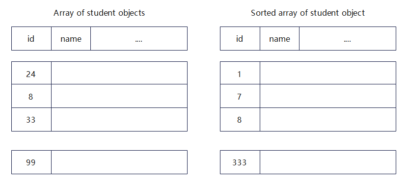
Example: UoA student records stored as an array
Issues
Depending on how data is organized, you get very different performance. We will study several alternatives and compare them.
Since we need to compare data structures and algorithms, we will consider a mathematical technique to determine their worst case performance without actually having to implement and run these algorithms
Why sort?
We already saw the benefit of searching for information in already-sorted data:
- Using binary search over sequential search
- Using a binary search tree over a BFS/DFS
Imagine trying to find a word in the dictionary, or looking up a phone number in the telephone book, if they were not sorted!
While computers can process large amounts of information faster than humans, it is still inefficient for the computer if the data is not sorted.
Here is a neat interactive website with excellent animations
Comparing: the precursor to sorting
Comparing two numbers:
int left = 23;
int right = 45;
if ((left - right) < 0) {
    System.out.println(left + " is smaller than " + right);
}
Comparing two strings uses exactly the same concept:
String left = "Catwoman";
String right = "Hulk";
if (left.compareTo(right) < 0) {
    System.out.println(left + " is before " + right);
}
The string’s compareTo() function does the “difference”calculation
0 means they are the same, negative means left is smaller than right, and positive means left is larger than right.
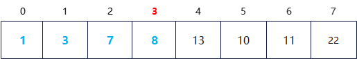
Selection sort
Sort the list one index at a time, by scanning ahead and selecting the smallest value in the remaining range
- Unsorted list
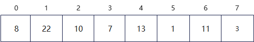
- Index 0, range [0:7]
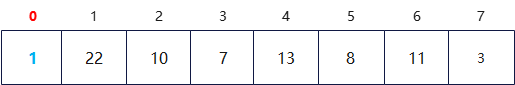
- Index 1, range [1:7]
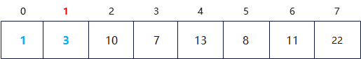
- Index 2, range [2:7]
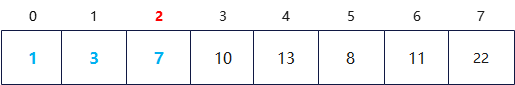
- Index 3, range [3:7]
- …
public void selectionSort(int array[], int n) {
    for (int i = 0; i < n-1; i++) {
        int least = i;
        for (int j = i+1; j < n; j++) {
            if (array[j] < array[least]) {
                least = j;
            }
        }
        swap(array[i], array[least]);
    }
}
A simple algorithm, but it essentially compares every element with every other element (even if the array is already sorted).
This will be expensive as the number of elements increases.
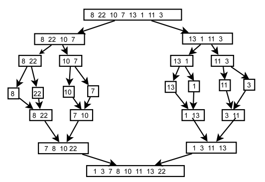
Merge sort
Merging 2 sorted lists
The problem with selection and insertion sort is they possibly require a quadratic amount of comparisons and movements. Can we do better?
Assume we have two already-sortedlists, and we merge them to produce a bigger sorted list
{7, 8, 10, 22}and{1, 3, 11, 13}- becomes
{1, 3, 7, 8, 10, 11, 13, 22} - The merging can be done easily at linear comparisons and movement
This is the idea behind mergesort, where we (recursively) break the array into halves, then merge the sorted halves together again.
Note: first and last in the following slide refers to indexes (not values)
Merge sort
public void mergeSort(int array[], int first, int last) {
    if (first < last) {
        int mid = (first+last) / 2;
        mergeSort(array, first, mid);
        mergeSort(array, mid+1, last);
        merge(array, first, last);
    }
}
Array complexity
-
Adding a new element: O(N), copying all elements to a larger array
-
Deleting an element: O(N) if in middle/front, O(1) at the end
-
Retrieving an element at a particular index: O(1)
Array list/vectors complexity
- Adding new value: O(1) amortised (on average) if doubling size… N insertions, and doubling array k times, to fit N elements (so N \(\approx\) 2k)
- Total cost: \(N + 2^1 + 2^2 + 2^3 + ... + 2^{k-1} + 2^k \\\rightarrow N + 2\times2^k (since \sum(2^1 + 2^2 + 2^3 + ... + 2^{k-1}) \approx 2^k) \\\rightarrow N + 2N \\\rightarrow O(N)\)
- The total cost is O(N), amprtised to O(1) over N operations
Linked-list complexity
-
Add/delete at front: O(1)
-
Add/delete at end, without knowing tail: O(N)
-
Add at end, with knowing tail: O(1)
-
Delete at end, with knowing tail, without access to prev node: O(N)
-
Delete at end, with knowing tail, with access to prev node: O(1)
-
Add/delete in middle: O(N)
-
Retrieving an element at a particular index: O(N)
Searching
Sequential:
- Elements not sorted, on average searching half the collection, O(N)
Binary search:
- Elements are sorted, eliminate half the search space at a time, O(logN)
Arbitrary code
if-statement, fixed number-of-step statements: O(1)
if (a < b) {
    tmp = a;
    a = b;
    b = tmp;
}
for-loop, while-loop, with linear steps: O(N)
for (i = 0; i < N; i += 2)
for-loop, while-loop, with dividing/multiplying steps: O(logN)
for (i = 1; i < N; i*=2)
nested for-loop, linear steps: O(\(N^2\))
for (i = 0; i < N; i+=2)
    for (j = 0; j < N; j++)
for-loop with function call… in this example: O(\(N^2\)logN)
for (i = 0; i < N; i+=2)  // O(N)
    mergeSort(list);      // O(NlogN)
nested for-loop with function call… in this example: O(\(N^2\)logN)
for (i = 0; i < N; i++)           // O(N)
    for (j = 1; j < N; j*=2)      // O(logN)
        merge(sortedA, sortedB);  // O(N)
Example: Determining if N is a prime
public boolean isPrime(int N) {
    for (int i = 2; i < N; i++) {
        if (N % i == 0)
            return false;
        }
    return true;
}
In worst case, we perform N-2 comparisons
This algorithm is O(N)
Assume each comparison take 1ms:
| N | 5 | 1009 | 10859 | 1495717 | 6428291 | 12518449 |
|---|---|---|---|---|---|---|
| Time O(N) | 3ms | 1s | 10.9s | 25mins | 1:47hrs | 3:29hrs |
We can obviously eliminate all even numbers… how does this help?
public boolean isPrime(int N) {
    for (int i = 3; i < N-1; i += 2) {
        if (N % i == 0)
            return false;
        }
    return true;
}
In worst case, we perform \(\frac{N-3}{2}\) comparisons
But this algorithm is still O(N), the \(\frac{1}{2}\) is just a constant factor andhas no dramatic influence on the overall complexity
| N | 5 | 1009 | 10859 | 1495717 | 6428291 | 12518449 |
|---|---|---|---|---|---|---|
| Time O(N) | 3ms | 1s | 10.9s | 25mins | 1:47hrs | 3:29hrs |
| Time O(\(\frac{N}{2}\)) | 1ms | 0.5s | 5.4s | 13mins | 0:54hrs | 1:45hrs |
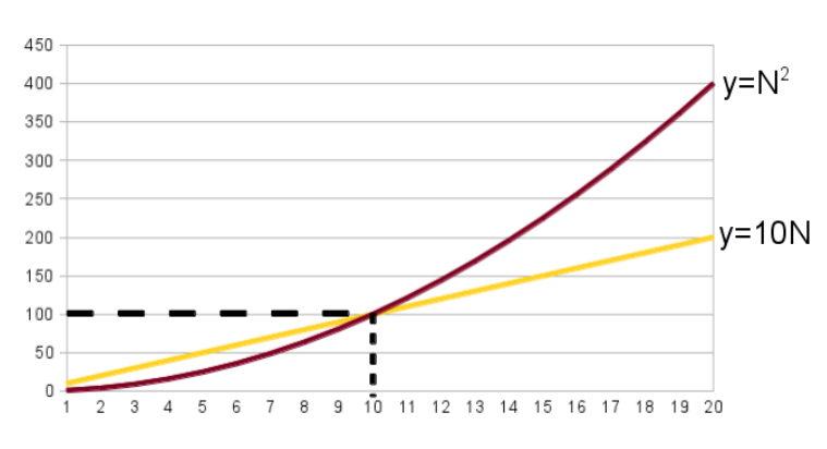
What do you mean the “factor” doesn’t matter?
Let’s compare 2 equations:
- \(y = 10N\).
- \(y = N^2\).
Despite the factor “10”, the second equation will eventually exceed the first equation. Even if we increase this to 100N or 200,000N,eventually the O(\(N^2\)) function will exceed it (with higher N values).
Therefore,O(N) is better than O(\(N^2\)) for sufficiently large N values
Analysis of algorithms
It provides techniques to compare algorithms without obtaining running times
/**
 * Algorithm arrayMax(A, n)
 * Input: an array A of n integers
 * Output: maximum element of A
 */

currentMax = A[0]
for (int i = 0; i < n; i++) {
    if (currentMax < A[i]) {
        currentMax = A[i];
    }
}
return currentMax;
Counting primitive operations
These are operations performed by an algorithm that is independent of the programming language and machine used. Each primitive operation corresponds to a low level instruction (which is a constant).
- Assigning a value to a variable.
- Calling a method.
- Performing an arithmetic operation.
- Comparing two numbers.
- Indexing into an array
Primitive operations in arrayMax
-
Initializing
currentMaxtoA[0]corresponds to 2 primitive operations: indexing into the array and assigning. -
Initializing
ito 1 at the beginning of for loop: one primitive operation. -
The comparison
i < nis done n times before entering the for loop: this amounts to n primitive operations. -
The body is executed (n-1) times. In each iteration there are either 4 (best case) and or 6 (worst case) operations.
Hence the number of primitive operations:
- \(T(n) = 2 + 1 + n + 4\times(n−1) + 1 = 5n\) (best case)
- \(T(n) = 2 + 1 + n + 6\times(n−1) + 1 = 7n − 3\) (worst case)
Asymptotic Notation
Is such detailed analysis necessary?
We are interested to compare the rate of growth of an algorithm as a function of its input sizen.
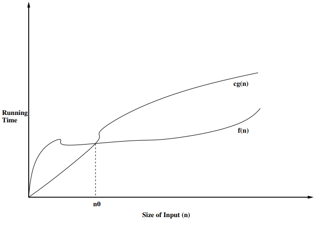
Definition
Let f(n) and g(n) be functions mapping non negative integers to real numbers. f(n) is said to be O(g(n)) (f(n) is order g(n)) if there is a real constant c and an integer constant \(n_0\) \(\geq\) 1 such that f(n) \(\leq\) c \(\times\) g(n) for every integern \(\geq\) \(n_0\)
Examples
-
\(f(n) =7n − 3\) is O(n): If you choose any c \(\geq\) 7 ands \(n_0\) = 1 then g(n) \(\geq\) f(n) for all n \(\geq\) 1.
-
\(20n^3 + 10nlogn + 5\) is O(\(n^3\)): \(20n^3 + 10nlogn + 5 \leq 35n^3\) for all n \(\geq\) 1.
\(2^{100}\) is O(1): \(2^{100} \leq 2^{100} \times\) 1 for n \(\geq\) 1
| logarithmic | linear | quadritic | polynomial | exponential |
|---|---|---|---|---|
| O(logn) | O(n) | O(\(n^3\)) | O(\(n^k\)): k \(\geq\)1 | O(\(a^n\)): a > 1 |
- Selection sort: \(O(N^2)\)
- Merge sort: \(O(NlogN)\)
- \(O(logN)\) recursive decomposition steps
Quick sort
It is a recursive sorting program. Key Idea:
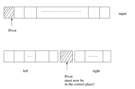
Use the pivot element to split the list into two parts:
- All elements to the left of the pivot are \(\leq\) the pivot element.
- All elements to the right of the pivot are > the pivot element.
The pivot is placed in between them.
Now recursively apply this idea to each of the left and the right parts. Stop the recursion when a part is of length 1
Splitting a list using the pivot
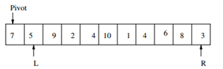
- Move L rightwards until an element is found that is > pivot; mark it.
- Move R leftwards until an element is found that is \(\leq\) pivot; mark it.
- Swap marked elements.
- Stop when L and R pass each other. Now swap (L,R) element with pivot. If this element is grater than pivot then swap with the element to the left of( L,R) element.
Example
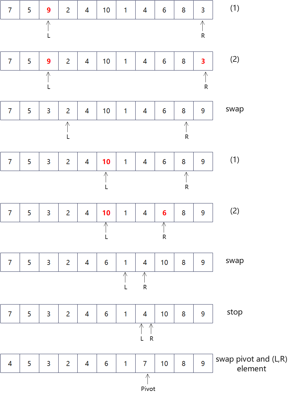
Split function and loop invariants
Split Function:
- Move L until A[L] > pivot element; mark A[L]; swap if A[R] is marked.
- Move R until A[R] \(\leq\) pivot element; mark A[R]; swap if A[L] ismarked.
- Repeat (1) and (2) for as long as L\(\neq\)R. When L=R, swap A[R] or A[R-1] as appropriate with the pivot. call QuickSort with input A[j..i]
Invariants:
While in (1) elements to the left of L are \(\leq\) the pivot (except the pivot itself). While in (2) elements to the right of R are > pivot. At the end of swap, the above two will hold for the elements at L and R. (Proof by induction on the length of the left and right parts). At exit from the splitloop invariants guarantee: left part \(\leq\) pivot < right part
Complexity of QuickSort
If the input array is of length k split makes about k comparisons to produce a left part and right part of length at most k-1. In the worst case the total number of comparisons is: \(\\k + (k-1) + (k-2) + ... + 1 = \frac{k\times(k+1)}{2} = O(k^2)\)
So, QuickSort is in the worst case O(\(n^2\))for input size n.
Average case complexity of QuickSort
If split yields approximately two equal length lists of length \(\frac{k-1}{2}\). \(T(n) = 2\times T(\frac{n}{2}) + n\) This is known as a recurrence relation. How to solve this?
\[T(1) = 1\\T(n) =2\times T(\frac{n}{2}) + bn \\= 2[2T(\frac{n}{4}) + \frac{bn}{2}] + bn\\= 4T[\frac{n}{4}] + \frac{2bn}{2} + bn\]Continuing in this manner of substitution, we will finally arrive at:\(T(n) = bn + \frac{bn}{2} + \frac{bn}{4} + ... + nT(\frac{n}{n})\) How many additive terms are there? If \(2^P = n\) then \(P = log_2n\). Hence there are \(log_2n\) additive terms. Therefore \(T(n) \leq bn log_2n\). Therefore the average case complexity of QuickSort is \(O(nlog_2n)\)
Conclusions
- We learnt about algorithms and their complexity
- We considered the O notation.
- Learnt about recursive algorithms
- Considered several sorting algorithms
- Quick sort as a recursive program
- Studied the complexity of quick sort